Nightlife Economic Impact: Temporal Analysis

How Rideshare Trips Change by Hour Around NYC Nightlife Zones

Author

Hariprasad Reddy Kotakondla

Published

December 18, 2025

Executive Summary

This analysis examines 684 million rideshare trips across 36 months (January 2022–December 2024) to understand how nightlife zones reshape NYC’s transportation patterns. By linking NYC TLC trip data with 2,058 Yelp-identified nightlife venues, I reveal that nightlife zones—representing only 26.6% of taxi zones—capture 51% of all trips and 53.9% of total revenue. During nighttime hours (8 PM–4 AM), this concentration intensifies to 61.1% of citywide revenue. The surge index peaks at 2 AM, when nightlife zones capture 24% more trips than their daily average, demonstrating that nightlife fundamentally reshapes when and where the city moves.

Statistical rigor: Bootstrap confidence intervals quantify uncertainty around key findings, permutation tests confirm significant differences between zone types (p < 0.001), sensitivity analysis demonstrates robustness across venue threshold choices, and a random forest predictive model validates the explanatory power of nightlife zone classification.

Introduction

Project Context

This individual report is part of the Nightlife Analytics: The Economics of Cities After Dark group project for STA 9750. Our team examines how nightlife activity impacts New York City across multiple dimensions. The full group summary report is available at: Group Project Report.

Overarching Question (OQ): How does nightlife activity—bars, entertainment, and rideshares—drive NYC economies and affect city safety and life quality?

My Specific Question (SQ): How do rideshare trip volumes change by hour in nightlife zones compared to the rest of NYC?

This analysis directly supports the OQ by quantifying the temporal dynamics of nightlife-driven transportation demand. Understanding when and where nightlife generates rideshare activity reveals the economic footprint of after-dark entertainment and informs transportation planning, driver positioning strategies, and urban policy decisions.

Key Innovation

Unlike traditional analyses that simply compare daytime versus nighttime patterns, this study introduces a surge index that quantifies relative nightlife dominance across each hour of the day. By measuring how much nightlife zones exceed their average trip share at different times, the surge index reveals the precise hours when nightlife districts become transportation hotspots—providing actionable insights for drivers, planners, and policymakers.

Why This Matters

Nightlife districts are economic engines generating jobs, tax revenue, and urban vitality. Understanding the relationship between nightlife density and rideshare patterns is essential for:

Transportation Planning: Optimizing service allocation during peak nightlife hours
Driver Strategy: Identifying high-revenue positioning opportunities
Economic Policy: Quantifying nightlife’s contribution to the transportation economy
Urban Planning: Informing infrastructure investments in entertainment districts

Methodology Overview

This analysis combines two primary data sources:

NYC TLC HVFHV Trip Records: High-volume for-hire vehicle (Uber/Lyft) trip data from January 2022 through December 2024, encompassing over 684 million individual trips.
Yelp Fusion API: Venue data for nightlife establishments (bars, lounges, dance clubs, music venues, cocktail bars) across NYC neighborhoods.

Nightlife Zone Definition: A taxi zone qualifies as a “nightlife zone” if it contains ≥5 nightlife venues. This threshold identifies zones with meaningful nightlife concentration while remaining robust to venue data incompleteness.

Nightlife Hours Definition: 8 PM to 4 AM, capturing the core window of evening entertainment activity.

Part 1: Data Acquisition

NYC TLC Trip Data

The NYC Taxi and Limousine Commission publishes monthly parquet files containing all high-volume for-hire vehicle trips. The following code downloads these files programmatically:

Show Code

# =============================================================================
# TLC DATA DOWNLOAD
# Programmatically download HVFHV parquet files from NYC TLC
# =============================================================================

# Create data directory structure
data_path <- "data/Nightlife_Rideshare_Analysis"
dir.create(data_path, showWarnings = FALSE, recursive = TRUE)

# Define date range for analysis
years <- 2022:2024
months <- sprintf("%02d", 1:12)

# Base URL for TLC data
base_url <- "https://d37ci6vzurychx.cloudfront.net/trip-data"

# Download each monthly file
for (year in years) {
  for (month in months) {
    file_name <- paste0("fhvhv_tripdata_", year, "-", month, ".parquet")
    file_url <- paste(base_url, file_name, sep = "/")
    dest_file <- file.path(data_path, file_name)
    
    # Only download if file doesn't exist
    if (!file.exists(dest_file)) {
      message("Downloading: ", file_name)
      tryCatch({
        download.file(file_url, dest_file, mode = "wb", quiet = TRUE)
      }, error = function(e) {
        message("Failed to download: ", file_name)
      })
    }
  }
}

message("TLC data download complete.")

Yelp API Venue Data

Nightlife venues were identified using the Yelp Fusion API. The following code queries the API across multiple NYC neighborhoods and nightlife categories:

Show Code

# =============================================================================
# YELP API DATA COLLECTION
# Fetch nightlife venue data from Yelp Fusion API
# =============================================================================

fetch_yelp_venues <- function(api_key) {
  if (api_key == "" || is.null(api_key)) {
    stop("Yelp API key not found. Set YELP_API_KEY environment variable.")
  }
  
  base_url <- "https://api.yelp.com/v3/businesses/search"
  all_venues <- tibble()
  
  # Target neighborhoods with known nightlife activity
  neighborhoods <- c(
    "East Village, NY", "West Village, NY", "Lower East Side, NY",
    "Williamsburg, Brooklyn", "Midtown Manhattan, NY", "Hell's Kitchen, NY",
    "Astoria, Queens", "Park Slope, Brooklyn", "SoHo, NY", "Bushwick, Brooklyn"
  )
  
  # Nightlife-specific Yelp categories
  categories <- c("bars", "lounges", "danceclubs", "musicvenues", "cocktailbars")
  
  for (hood in neighborhoods) {
    for (cat in categories) {
      for (offset in seq(0, 50, by = 50)) {
        tryCatch({
          response <- GET(
            base_url,
            add_headers(Authorization = paste("Bearer", api_key)),
            query = list(
              location = hood,
              categories = cat,
              limit = 50,
              offset = offset
            ),
            timeout(30)
          )
          
          if (status_code(response) != 200) break
          
          data <- content(response, as = "parsed")
          if (length(data$businesses) == 0) break
          
          venues <- tibble(
            id = map_chr(data$businesses, ~.x$id),
            name = map_chr(data$businesses, ~.x$name),
            latitude = map_dbl(data$businesses, ~.x$coordinates$latitude),
            longitude = map_dbl(data$businesses, ~.x$coordinates$longitude),
            rating = map_dbl(data$businesses, ~.x$rating),
            review_count = map_int(data$businesses, ~.x$review_count),
            categories = map_chr(data$businesses, 
                                 ~paste(map_chr(.x$categories, ~.x$title), collapse = ", "))
          )
          
          all_venues <- bind_rows(all_venues, venues)
          Sys.sleep(0.2)  # Rate limiting
        }, error = function(e) {
          message("API error for ", hood, " - ", cat)
        })
      }
    }
  }
  
  return(all_venues %>% distinct(id, .keep_all = TRUE))
}

# Fetch venues using API key from environment variable
YELP_API_KEY <- Sys.getenv("YELP_API_KEY")
nightlife_venues <- fetch_yelp_venues(YELP_API_KEY)

# Cache results for reproducibility
write_csv(nightlife_venues, "nightlife_venues_cached.csv")

NYC Taxi Zone Boundaries

Taxi zone shapefiles are downloaded from NYC Open Data:

Show Code

# Download taxi zone shapefile from NYC Open Data
taxi_zone_url <- "https://d37ci6vzurychx.cloudfront.net/misc/taxi_zones.zip"
download.file(taxi_zone_url, "taxi_zones.zip", mode = "wb")
unzip("taxi_zones.zip", exdir = ".")

Part 2: Data Quality Assessment

Sampling Quality

TLC Data: The NYC TLC dataset is comprehensive, containing every recorded HVFHV trip in the city. There are no sampling concerns—this is population data, not a sample. However, trips that were cancelled, not recorded due to technical issues, or occurred in unlicensed vehicles are not captured.

Yelp Data: The Yelp dataset represents venues with active Yelp business profiles. This introduces potential undercoverage for:

Establishments that don’t maintain Yelp profiles
Newly opened venues not yet indexed
Cash-only or informal establishments less likely to appear online

Despite these limitations, Yelp provides the most comprehensive publicly-available database of nightlife venues with precise geocoding.

Recording Quality

TLC Data Quality Checks:

Trip records include pickup/dropoff times, locations (taxi zone IDs), and fare components
Base passenger fare is computed as the sum of base fare, tolls, fees, and surcharges
Tips data is incomplete for cash payments (a known limitation)
Location IDs are standardized to NYC taxi zone boundaries

Yelp Data Quality Checks:

All venues have valid coordinates (required for API response)
16 venues fell outside NYC taxi zone boundaries and were excluded
Rating and review counts provide quality signals but were not used for filtering

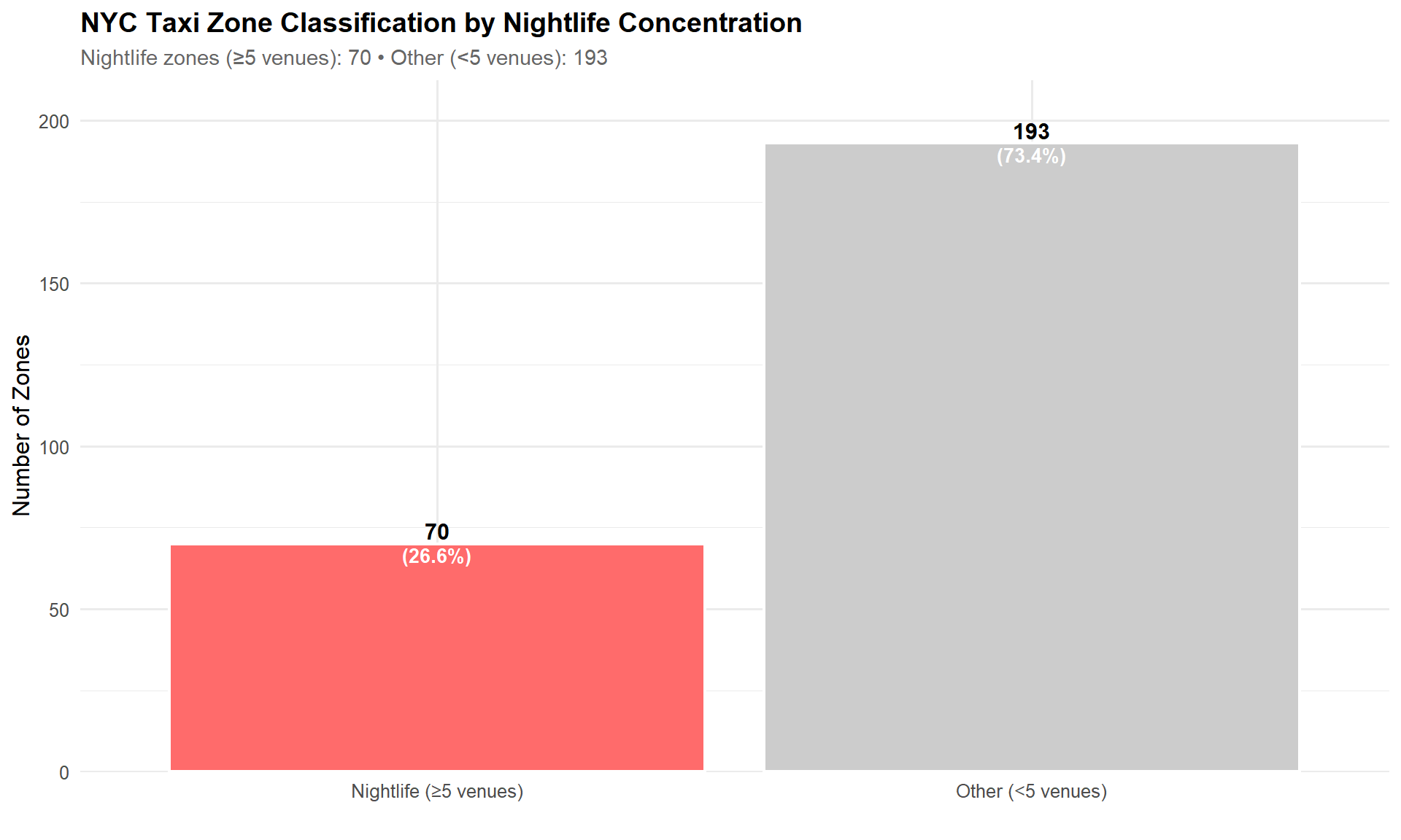
We identified 2,058 nightlife venues across NYC taxi zones (16 venues excluded as they fall outside taxi zone boundaries). After spatial joining, 70 zones (26.6%) qualify as nightlife zones.

Part 3: Where is Nightlife?

Chart 1: Zone Coverage

Show Code

# Compute zone classification counts
zone_counts <- taxi_zones_sf %>%
  st_drop_geometry() %>%
  count(zone_type, name = "Count") %>%
  mutate(
    zone_type = factor(zone_type, levels = c("Nightlife (≥5 venues)", "Other (<5 venues)")),
    pct = round(100 * Count / total_zones, 1)
  )

ggplot(zone_counts, aes(x = zone_type, y = Count, fill = zone_type)) +
  geom_col(color = "white", linewidth = 0.8) +
  geom_text(aes(label = Count), vjust = -0.3, fontface = "bold", size = 4) +
  geom_text(aes(label = paste0("(", pct, "%)")), vjust = 1.2, color = "white", 
            fontface = "bold", size = 3.5) +
  scale_fill_manual(
    values = c("Nightlife (≥5 venues)" = colors$nightlife, "Other (<5 venues)" = colors$gray),
    guide = "none"
  ) +
  scale_y_continuous(expand = expansion(mult = c(0, 0.1))) +
  labs(
    title = "NYC Taxi Zone Classification by Nightlife Concentration",
    subtitle = paste0("Nightlife zones (≥5 venues): ", n_nightlife_zones, 
                      " • Other (<5 venues): ", total_zones - n_nightlife_zones),
    x = "", y = "Number of Zones"
  )

Although nightlife zones make up only 26.6% of NYC taxi zones, their share of trips and revenue is far larger, as we will demonstrate. This establishes that nightlife activity is spatially concentrated but economically influential.

Chart 2: Interactive Nightlife Zone Map

Show Code

# Transform to WGS84 for Leaflet
nightlife_leaflet <- taxi_zones_sf %>%
  st_transform(4326) %>%
  mutate(
    is_nightlife = n_venues >= 5,
    popup_text = paste0(
      "<strong>", Zone, "</strong><br>",
      "Borough: ", Borough, "<br>",
      "Venues: ", n_venues, "<br>",
      ifelse(n_venues >= 5, 
             "<span style='color: #FF6B6B;'>✓ Nightlife Zone</span>",
             "<span style='color: gray;'>Not a nightlife zone</span>")
    )
  )

# Color palette for nightlife intensity
pal <- colorNumeric(
  palette = c("#FFCCBC", "#FF6B6B", "#C0392B", "#6A1B1B"),
  domain = c(5, max(nightlife_leaflet$n_venues[nightlife_leaflet$n_venues >= 5])),
  na.color = "#E8E8E8"
)

# Build interactive map
leaflet(nightlife_leaflet, height = 500) %>%
  addProviderTiles(providers$CartoDB.DarkMatter, 
                   options = providerTileOptions(opacity = 0.8)) %>%
  addPolygons(
    data = nightlife_leaflet %>% filter(!is_nightlife),
    fillColor = "#404040", fillOpacity = 0.3,
    color = "#606060", weight = 0.5,
    popup = ~popup_text,
    highlightOptions = highlightOptions(weight = 2, color = "#FFFFFF", fillOpacity = 0.5)
  ) %>%
  addPolygons(
    data = nightlife_leaflet %>% filter(is_nightlife),
    fillColor = ~pal(n_venues), fillOpacity = 0.7,
    color = "#FFFFFF", weight = 1,
    popup = ~popup_text,
    highlightOptions = highlightOptions(weight = 3, color = "#FFD700", fillOpacity = 0.9)
  ) %>%
  addLegend(position = "bottomright", pal = pal,
            values = nightlife_leaflet$n_venues[nightlife_leaflet$is_nightlife],
            title = "Nightlife Venues", opacity = 0.8) %>%
  addControl(
    html = "<div style='background: rgba(0,0,0,0.7); padding: 10px 15px; border-radius: 5px;'>
              <span style='color: #FF6B6B; font-size: 18px; font-weight: bold;'>
                NYC Nightlife Hotspots
              </span><br>
              <span style='color: #CCCCCC; font-size: 12px;'>
                Click zones for details. 70 zones with 5+ venues highlighted.
              </span>
            </div>",
    position = "topright"
  ) %>%
  setView(lng = -73.95, lat = 40.75, zoom = 11)

Interactive map: Click on any zone to see venue counts and classification. Nightlife venues cluster heavily in Lower Manhattan, East Village, and parts of Brooklyn, forming clear hotspots of nighttime movement.

Part 4: When Does Nightlife Demand Happen?

We analyzed 684,376,551 rideshare trips spanning 36 months (January 2022 to December 2024).

Nightlife zones (≥5 venues) capture 51% of trips and 53.9% of revenue, despite representing only 26.6% of taxi zones.

Chart 3: Hourly Trip Volume Comparison

Show Code

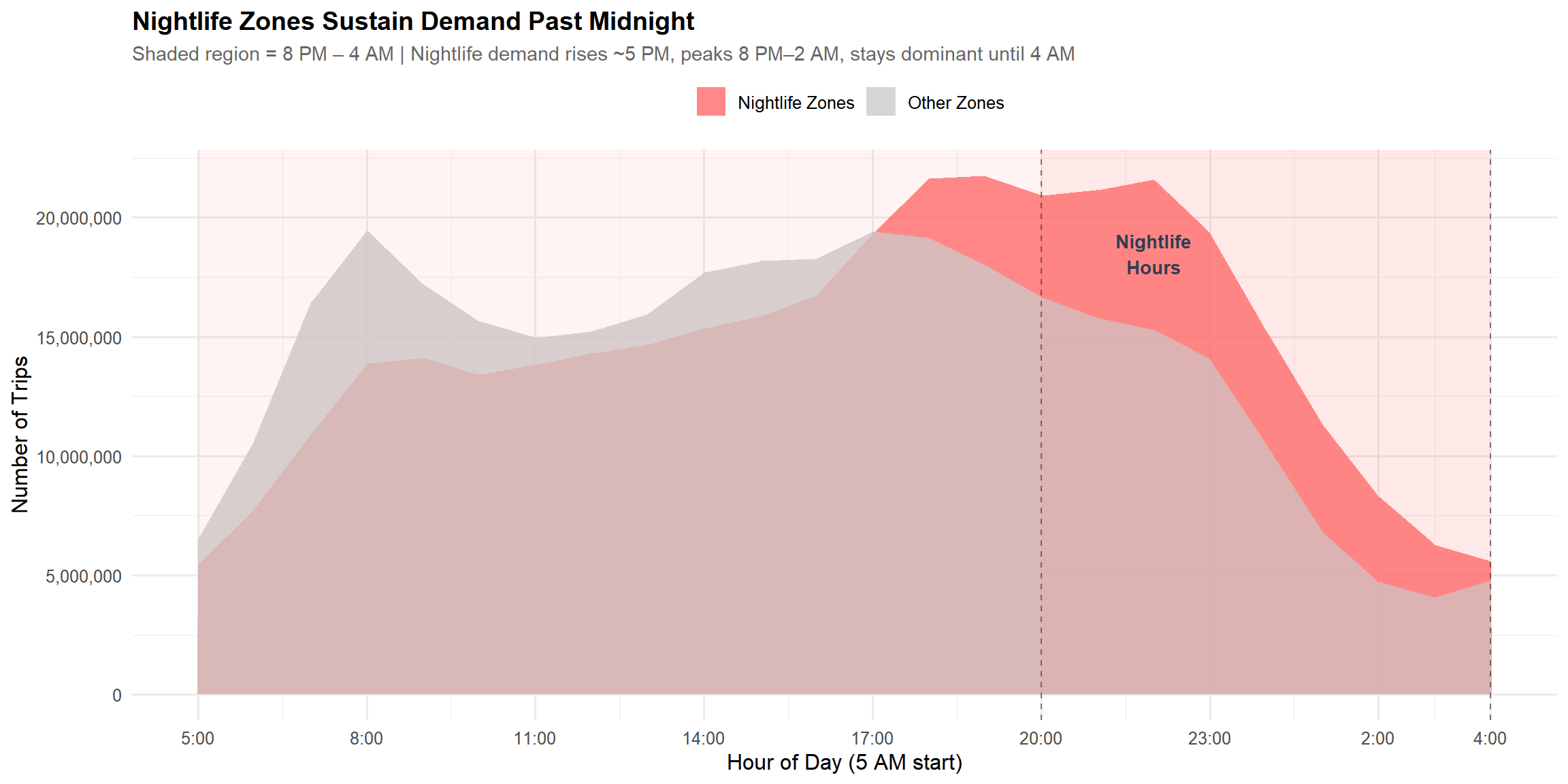
hourly_comparison <- tlc_with_zones %>%
  mutate(zone_group = if_else(zone_class == "Nightlife", "Nightlife Zones", "Other Zones")) %>%
  group_by(hour_reordered, zone_group) %>%
  summarise(trips = sum(trips), .groups = "drop")

ggplot(hourly_comparison, aes(x = hour_reordered, y = trips, fill = zone_group)) +
  geom_area(alpha = 0.8, position = "identity") +
  geom_vline(xintercept = c(reorder_hours_5am(4), reorder_hours_5am(20)), 
             linetype = "dashed", alpha = 0.5) +
  annotate("rect", xmin = reorder_hours_5am(20), xmax = 23, ymin = 0, ymax = Inf, 
           alpha = 0.08, fill = colors$nightlife) +
  annotate("rect", xmin = 0, xmax = reorder_hours_5am(4), ymin = 0, ymax = Inf, 
           alpha = 0.08, fill = colors$nightlife) +
  annotate("text", x = reorder_hours_5am(22), y = max(hourly_comparison$trips) * 0.85, 
           label = "Nightlife\nHours", fontface = "bold", size = 3.5, color = colors$night) +
  scale_fill_manual(values = c("Nightlife Zones" = colors$nightlife, "Other Zones" = colors$gray)) +
  scale_x_continuous(breaks = c(0, seq(3, 21, 3), 23), labels = function(x) hour_labels_5am(x)) +
  scale_y_continuous(labels = comma) +
  labs(
    title = "Nightlife Zones Sustain Demand Past Midnight",
    subtitle = "Shaded region = 8 PM – 4 AM | Nightlife demand rises ~5 PM, peaks 8 PM–2 AM, stays dominant until 4 AM",
    x = "Hour of Day (5 AM start)", y = "Number of Trips", fill = ""
  )

This chart directly answers my specific question. Nightlife zones sustain significantly higher trip volumes during the nighttime window (8 PM–4 AM). While “Other” zones drop sharply after 11 PM, nightlife zones remain the primary drivers of city mobility until closing hours. Nightlife clearly reshapes when the city moves.

Chart 4: Nightlife Surge Index

Show Code

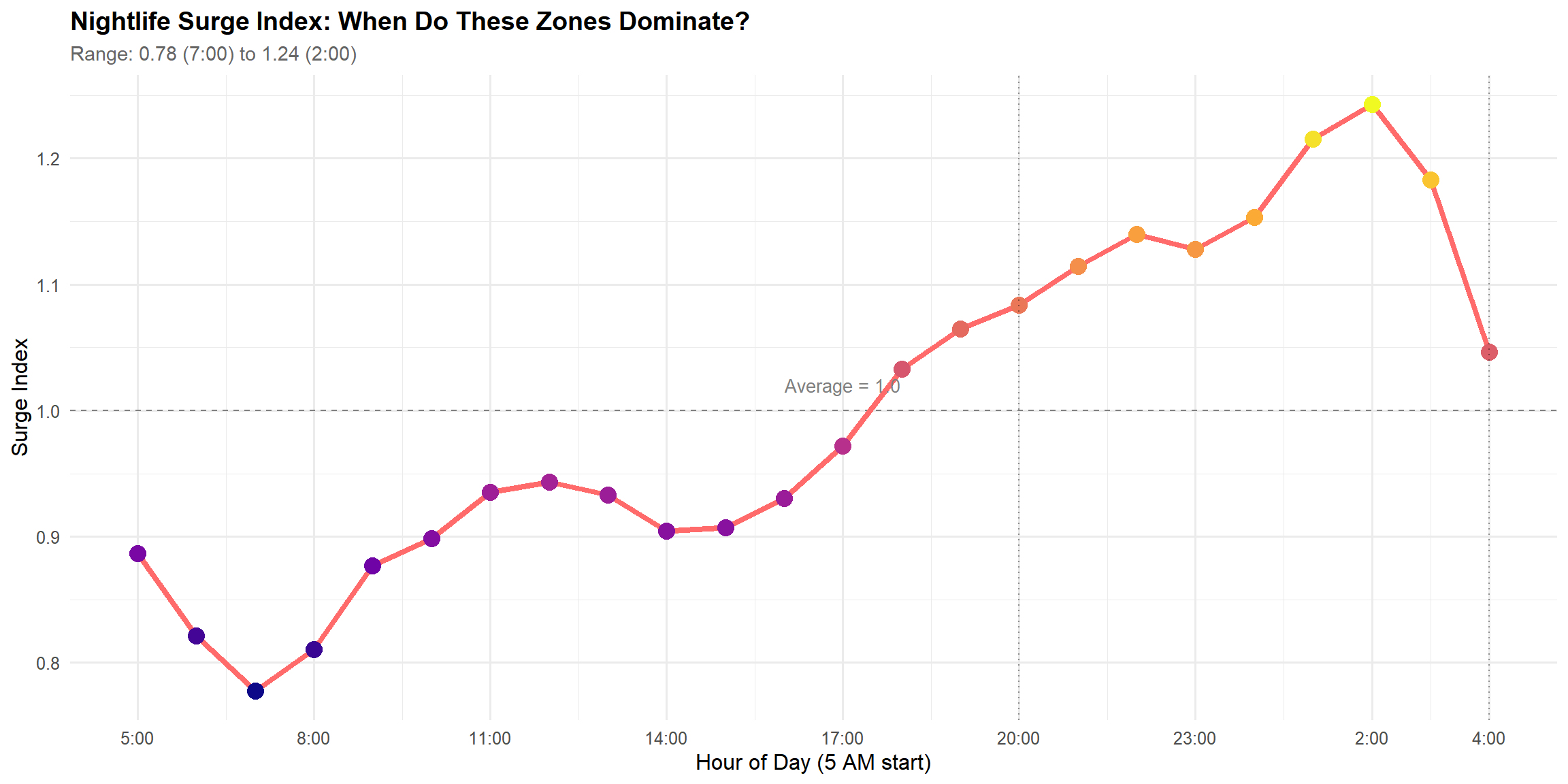
surge_data <- tlc_with_zones %>%
  group_by(pickup_hour) %>%
  summarise(
    total_trips = sum(trips),
    nightlife_trips = sum(trips[zone_class == "Nightlife"]),
    nightlife_share = nightlife_trips / total_trips,
    .groups = "drop"
  ) %>%
  mutate(
    surge_index = nightlife_share / mean(nightlife_share),
    hour_reordered = reorder_hours_5am(pickup_hour)
  )

peak_hour <- surge_data %>% filter(surge_index == max(surge_index)) %>% pull(pickup_hour)
peak_surge <- round(max(surge_data$surge_index), 2)
trough_hour <- surge_data %>% filter(surge_index == min(surge_index)) %>% pull(pickup_hour)
trough_surge <- round(min(surge_data$surge_index), 2)

ggplot(surge_data, aes(x = hour_reordered, y = surge_index)) +
  geom_hline(yintercept = 1, linetype = "dashed", color = "gray50") +
  geom_line(color = colors$nightlife, linewidth = 1.5) +
  geom_point(aes(color = surge_index), size = 4) +
  geom_vline(xintercept = c(reorder_hours_5am(4), reorder_hours_5am(20)), 
             linetype = "dotted", alpha = 0.4) +
  scale_color_viridis_c(option = "plasma", guide = "none") +
  scale_x_continuous(breaks = c(0, seq(3, 21, 3), 23), labels = function(x) hour_labels_5am(x)) +
  scale_y_continuous(breaks = seq(0.6, 1.6, 0.1)) +
  annotate("text", x = 12, y = 1.02, label = "Average = 1.0", color = "gray50", size = 3.5) +
  labs(
    title = "Nightlife Surge Index: When Do These Zones Dominate?",
    subtitle = paste0("Range: ", trough_surge, " (", trough_hour, ":00) to ", 
                      peak_surge, " (", peak_hour, ":00)"),
    x = "Hour of Day (5 AM start)", y = "Surge Index"
  )

The surge index quantifies nightlife zone dominance across the day. It peaks sharply at 2:00 AM (surge index = 1.24), when nightlife zones capture 24% more trips than their daily average share. This confirms that nightlife demand disproportionately drives late-night transportation needs.

Part 5: Revenue Analysis

Chart 5: Hour × Day Revenue Heatmaps

Show Code

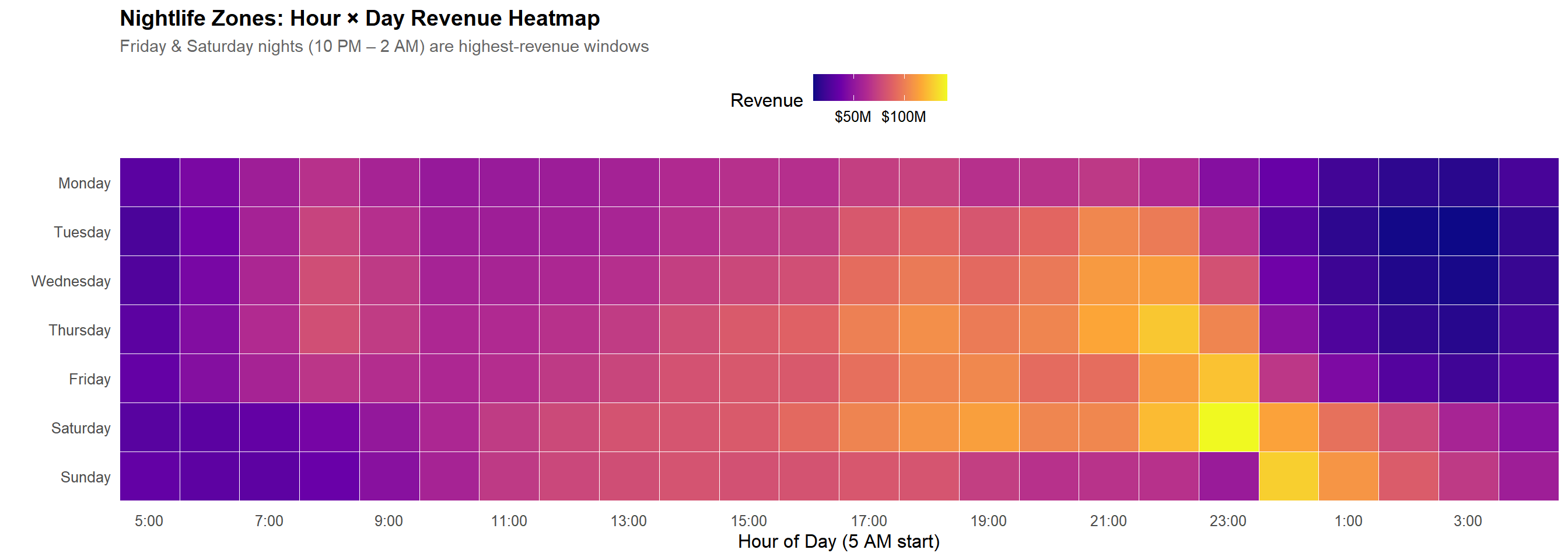
# Nightlife zones heatmap - Monday to Sunday order
hourly_dow_nightlife <- tlc_with_zones %>%
  filter(zone_class == "Nightlife") %>%
  group_by(pickup_hour, pickup_dow) %>%
  summarise(revenue = sum(total_fare, na.rm = TRUE), .groups = "drop") %>%
  mutate(
    pickup_dow = factor(pickup_dow, levels = c("Monday", "Tuesday", "Wednesday", 
                                                "Thursday", "Friday", "Saturday", "Sunday")),
    hour_reordered = reorder_hours_5am(pickup_hour)
  )

ggplot(hourly_dow_nightlife, aes(x = hour_reordered, y = pickup_dow, fill = revenue)) +
  geom_tile(color = "white", linewidth = 0.3) +
  scale_fill_viridis_c(option = "plasma", labels = dollar_format(scale = 1e-6, suffix = "M")) +
  scale_x_continuous(breaks = seq(0, 23, 2), labels = function(x) hour_labels_5am(x), expand = c(0, 0)) +
  scale_y_discrete(limits = rev)+
  labs(title = "Nightlife Zones: Hour × Day Revenue Heatmap",
       subtitle = "Friday & Saturday nights (10 PM – 2 AM) are highest-revenue windows",
       x = "Hour of Day (5 AM start)", y = "", fill = "Revenue") +
  theme(panel.grid = element_blank())

Show Code

# Other zones heatmap - Monday to Sunday order
hourly_dow_other <- tlc_with_zones %>%
  filter(zone_class == "Other") %>%
  group_by(pickup_hour, pickup_dow) %>%
  summarise(revenue = sum(total_fare, na.rm = TRUE), .groups = "drop") %>%
  mutate(
    pickup_dow = factor(pickup_dow, levels = c("Monday", "Tuesday", "Wednesday", 
                                                "Thursday", "Friday", "Saturday", "Sunday")),
    hour_reordered = reorder_hours_5am(pickup_hour)
  )

ggplot(hourly_dow_other, aes(x = hour_reordered, y = pickup_dow, fill = revenue)) +
  geom_tile(color = "white", linewidth = 0.3) +
  scale_fill_viridis_c(option = "viridis", labels = dollar_format(scale = 1e-6, suffix = "M")) +
  scale_x_continuous(breaks = seq(0, 23, 2), labels = function(x) hour_labels_5am(x), expand = c(0, 0)) +
  scale_y_discrete(limits = rev)+
  labs(title = "Other Zones: Hour × Day Revenue Heatmap",
       subtitle = "Peaks during daytime rush hours; drops sharply after midnight",
       x = "Hour of Day (5 AM start)", y = "", fill = "Revenue") +
  theme(panel.grid = element_blank())

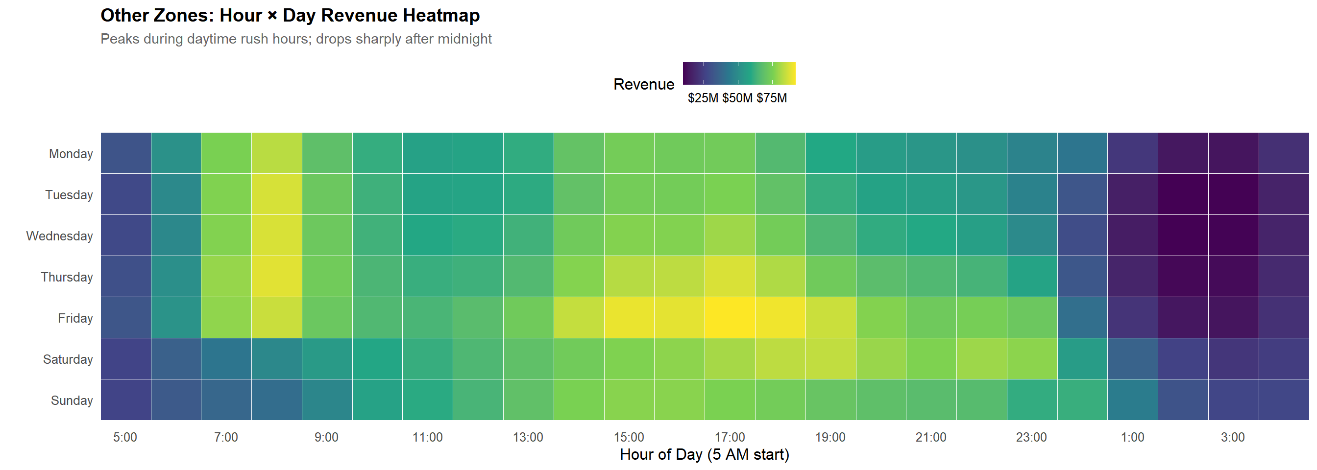
The contrast is striking: nightlife zones generate their highest revenue between 10 PM and 2 AM, while non-nightlife zones peak during traditional commuter hours (7–10 AM and 4–7 PM). This directly demonstrates that time-of-day usage differs dramatically across zone types.

Chart 6: Revenue Distribution by Zone Type and Time

Show Code

revenue_split <- tlc_with_zones %>%
  mutate(time_of_day = if_else(is_night, "Night (8 PM - 4 AM)", "Day (4 AM - 8 PM)")) %>%
  group_by(zone_class, time_of_day) %>%
  summarise(revenue = sum(total_fare, na.rm = TRUE), .groups = "drop") %>%
  mutate(zone_class = factor(zone_class, levels = c("Nightlife", "Other")))

revenue_split <- revenue_split %>%
  group_by(time_of_day) %>%
  mutate(pct = round(100 * revenue / sum(revenue), 1)) %>%
  ungroup()

night_nl_pct <- revenue_split %>% 
  filter(zone_class == "Nightlife", time_of_day == "Night (8 PM - 4 AM)") %>% 
  pull(pct)

ggplot(revenue_split, aes(x = time_of_day, y = revenue, fill = zone_class)) +
  geom_col(position = "dodge", color = "white", linewidth = 0.8) +
  geom_text(aes(label = paste0(pct, "%")), 
            position = position_dodge(0.9), vjust = -0.3, fontface = "bold", size = 3.5) +
  scale_fill_manual(values = c("Nightlife" = colors$nightlife, "Other" = colors$gray)) +
  scale_y_continuous(labels = dollar_format(scale = 1e-6, suffix = "M"), 
                     expand = expansion(mult = c(0, 0.15))) +
  labs(
    title = "Revenue Distribution: Nightlife vs Other Zones",
    subtitle = "Nightlife zones dominate both day and night revenue",
    x = "", y = "Revenue", fill = "Zone Type"
  )

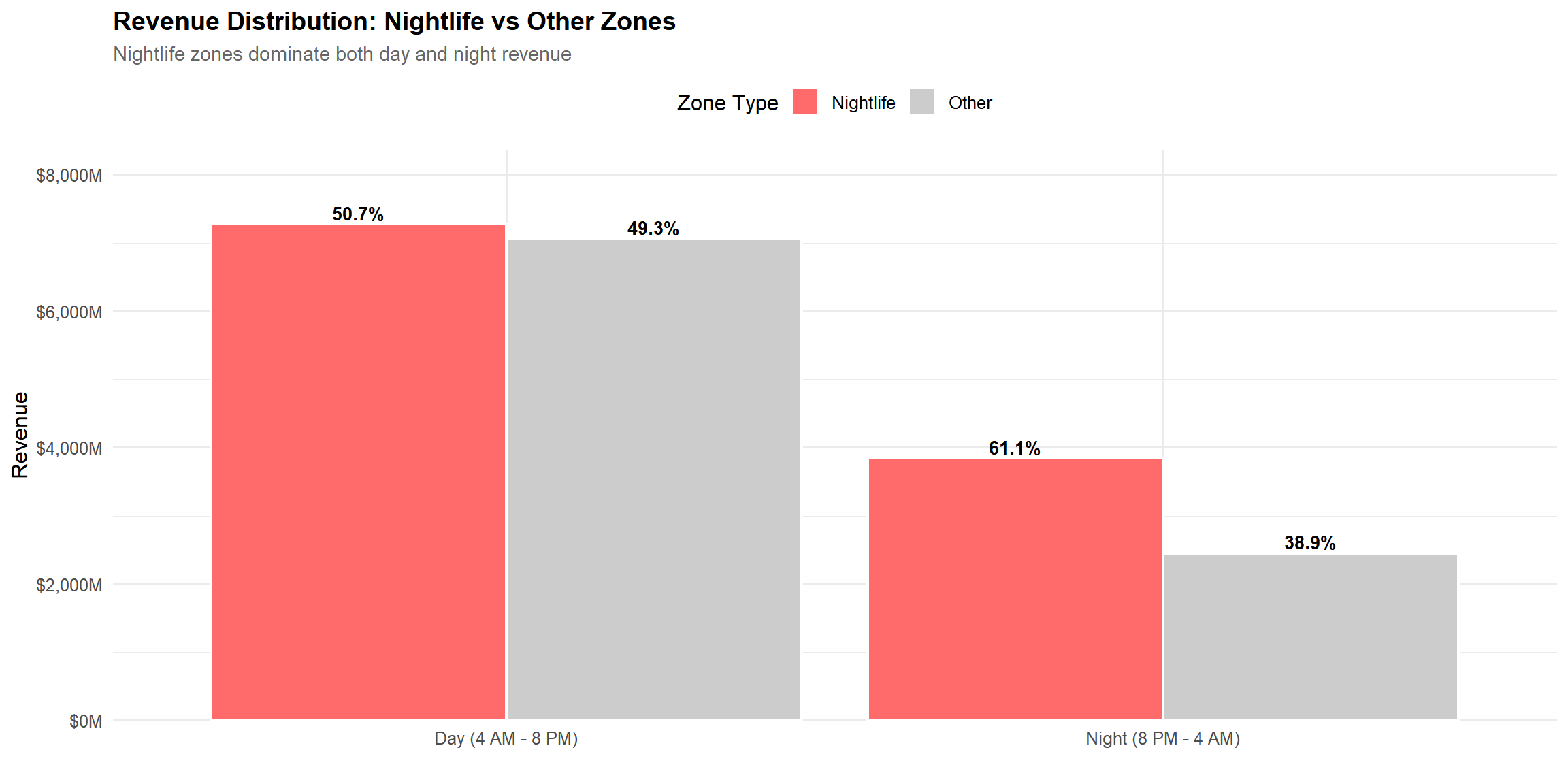
During nighttime hours, nightlife zones capture 61.1% of citywide revenue, far exceeding their 26.6% spatial footprint. Even during the day, nightlife zones remain economically strong, indicating that these districts serve as continuous activity hubs.

Part 6: Temporal Patterns

Chart 7: Day of Week Revenue

Show Code

dow_revenue <- tlc_with_zones %>%
  filter(zone_class == "Nightlife") %>%
  mutate(time_of_day = if_else(is_night, "Night (8 PM - 4 AM)", "Day (4 AM - 8 PM)")) %>%
  group_by(pickup_dow, time_of_day) %>%
  summarise(revenue = sum(total_fare, na.rm = TRUE), .groups = "drop") %>%
  mutate(pickup_dow = factor(pickup_dow, levels = c("Monday", "Tuesday", "Wednesday", 
                                                     "Thursday", "Friday", "Saturday", "Sunday")))

night_revenue <- dow_revenue %>% filter(time_of_day == "Night (8 PM - 4 AM)")
peak_night_row <- night_revenue %>% slice_max(revenue, n = 1)
peak_day <- as.character(peak_night_row$pickup_dow)
peak_night_rev <- peak_night_row$revenue

ggplot(dow_revenue, aes(x = pickup_dow, y = revenue, fill = time_of_day)) +
  geom_col(position = "dodge", color = "white", linewidth = 0.5) +
  scale_fill_manual(values = c("Night (8 PM - 4 AM)" = colors$night, 
                               "Day (4 AM - 8 PM)" = colors$day)) +
  scale_y_continuous(labels = dollar_format(scale = 1e-6, suffix = "M")) +
  labs(
    title = "Nightlife Zone Revenue: Day vs Night by Day of Week",
    subtitle = paste0("Peak night revenue: ", peak_day, " at $", round(peak_night_rev / 1e6, 1), "M"),
    x = "", y = "Revenue", fill = ""
  ) +
  theme(axis.text.x = element_text(angle = 45, hjust = 1))

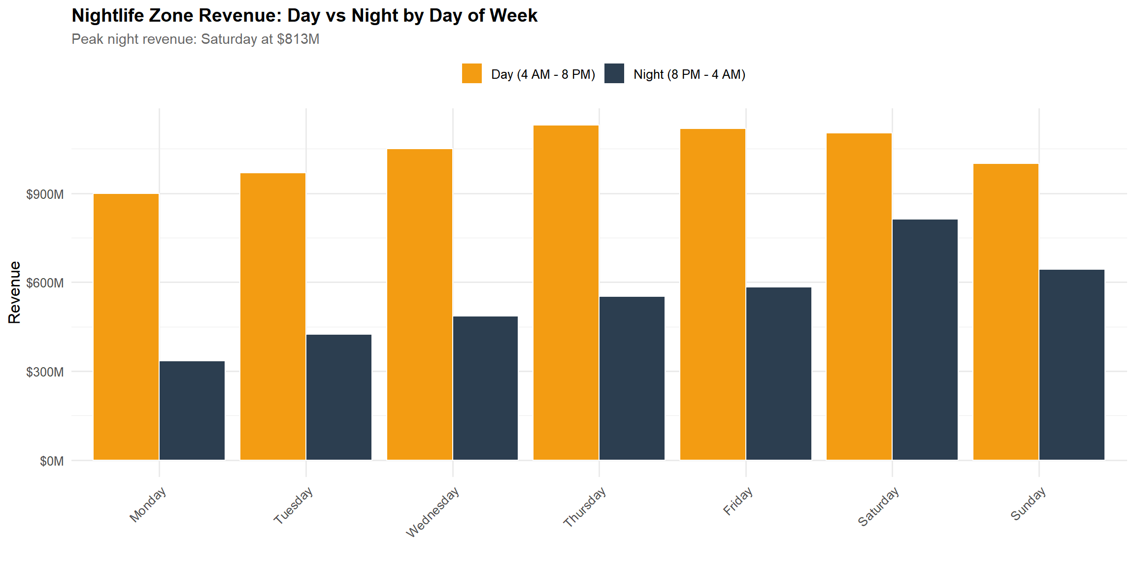
Weekend nights, especially Friday and Saturday, show the strongest nightlife revenue. This weekly rhythm mirrors cultural behavior and supports operational planning—rideshare supply can be aligned with predictable nightlife cycles.

Chart 8: Monthly Trends Over Time

Show Code

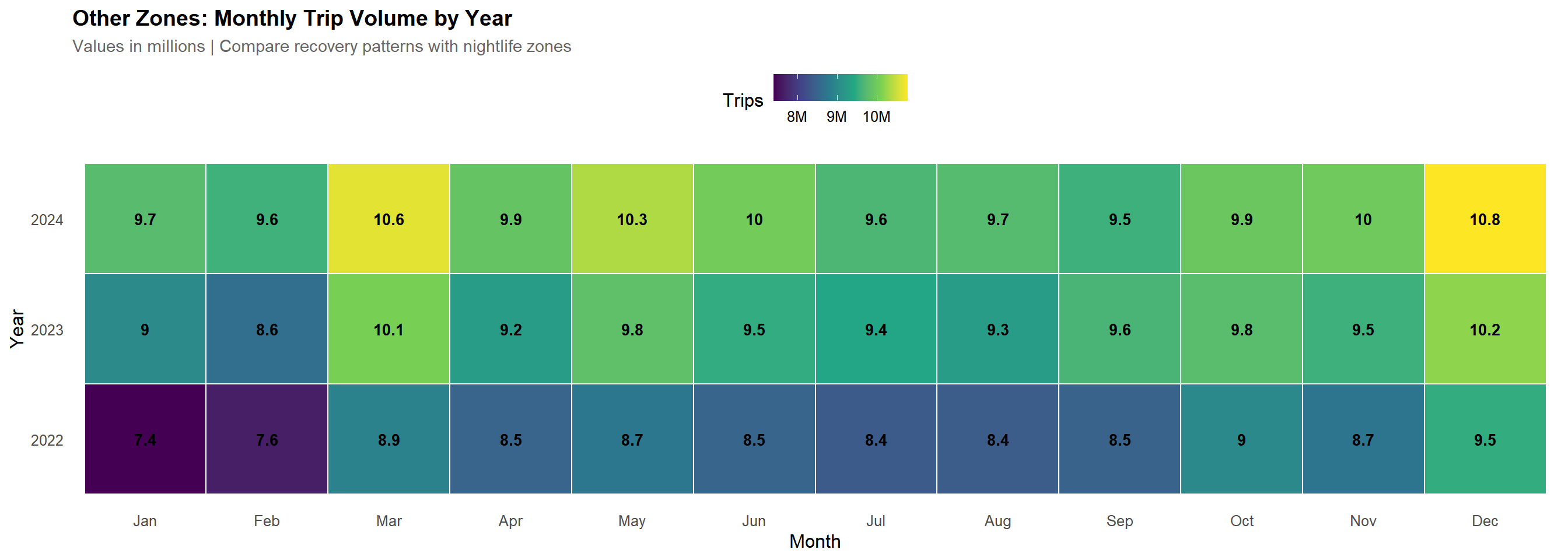
# Nightlife zones monthly heatmap
monthly_trips_nightlife <- tlc_with_zones %>%
  filter(zone_class == "Nightlife") %>%
  group_by(pickup_year, pickup_month) %>%
  summarise(trips = sum(trips), .groups = "drop") %>%
  mutate(
    month_name = factor(month.abb[pickup_month], levels = month.abb),
    pickup_year = factor(pickup_year)
  )

ggplot(monthly_trips_nightlife, aes(x = month_name, y = pickup_year, fill = trips)) +
  geom_tile(color = "white", linewidth = 0.5) +
  geom_text(aes(label = round(trips / 1e6, 1)), color = "black", size = 3.5, fontface = "bold") +
  scale_fill_viridis_c(option = "plasma", labels = label_number(scale = 1e-6, suffix = "M")) +
  labs(title = "Nightlife Zones: Monthly Trip Volume by Year",
       subtitle = "Values in millions | Shows recovery trajectory from 2022 onwards",
       x = "Month", y = "Year", fill = "Trips") +
  theme(panel.grid = element_blank())

Show Code

# Other zones monthly heatmap
monthly_trips_other <- tlc_with_zones %>%
  filter(zone_class == "Other") %>%
  group_by(pickup_year, pickup_month) %>%
  summarise(trips = sum(trips), .groups = "drop") %>%
  mutate(
    month_name = factor(month.abb[pickup_month], levels = month.abb),
    pickup_year = factor(pickup_year)
  )

ggplot(monthly_trips_other, aes(x = month_name, y = pickup_year, fill = trips)) +
  geom_tile(color = "white", linewidth = 0.5) +
  geom_text(aes(label = round(trips / 1e6, 1)), color = "black", size = 3.5, fontface = "bold") +
  scale_fill_viridis_c(option = "viridis", labels = label_number(scale = 1e-6, suffix = "M")) +
  labs(title = "Other Zones: Monthly Trip Volume by Year",
       subtitle = "Values in millions | Compare recovery patterns with nightlife zones",
       x = "Month", y = "Year", fill = "Trips") +
  theme(panel.grid = element_blank())

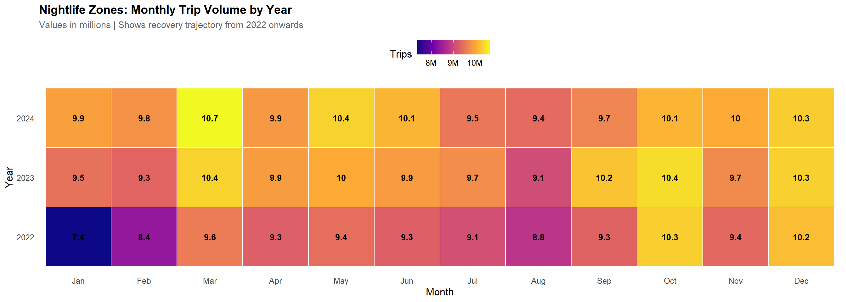
Monthly trip volumes show clear seasonality, with summer peaks and winter troughs. Both nightlife and other zones follow similar long-term patterns, indicating that hourly differences are not due to seasonal distortions but genuine behavioral differences across hours.

Part 7: Statistical Inference

This section moves beyond descriptive statistics to provide rigorous statistical inference, including bootstrap confidence intervals, permutation tests, sensitivity analysis, and predictive modeling.

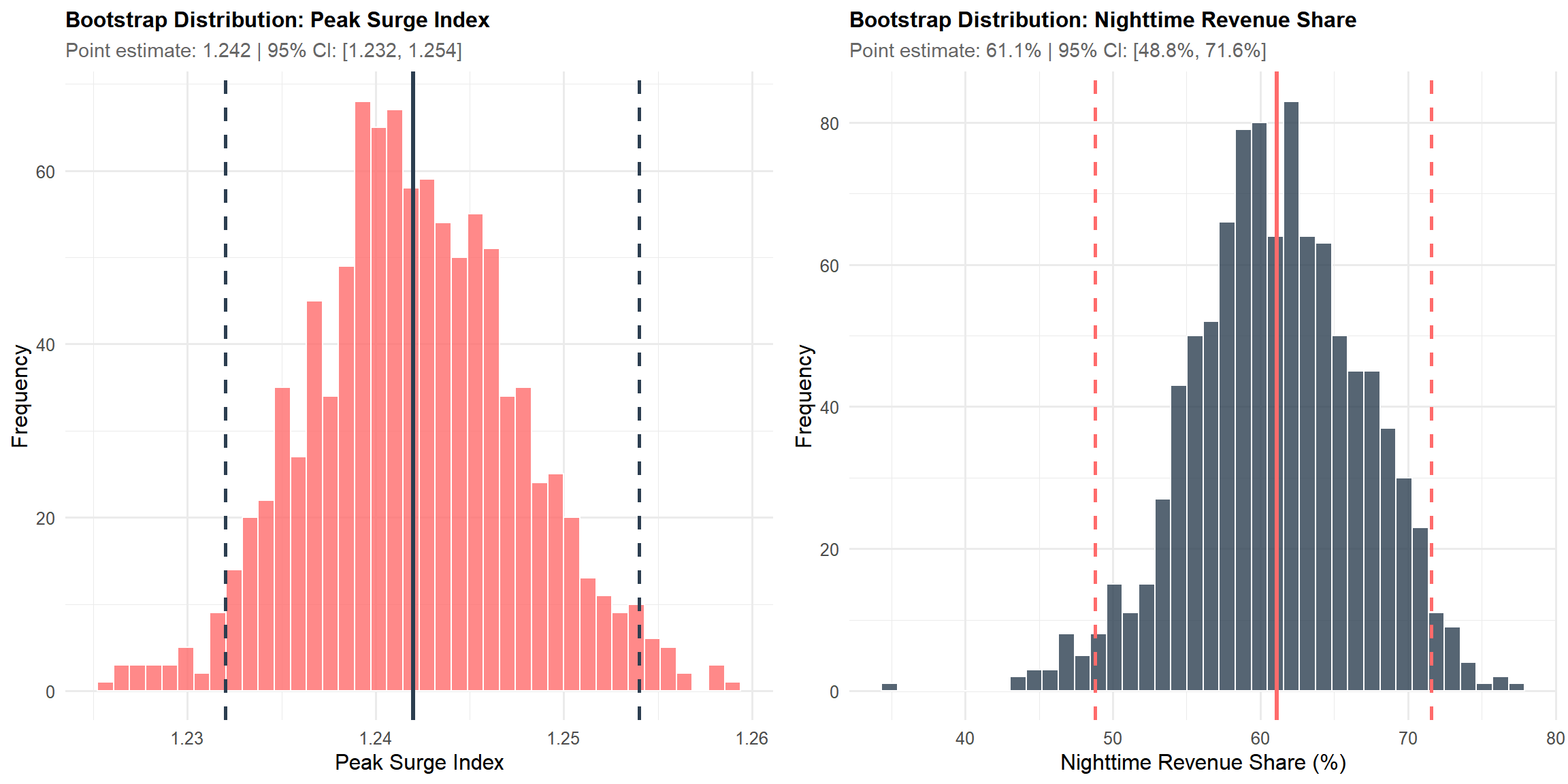
Bootstrap Confidence Intervals

To quantify uncertainty around key findings, we use bootstrap resampling to construct 95% confidence intervals for the peak surge index and nightlife revenue share.

Show Code

# =============================================================================
# BOOTSTRAP CONFIDENCE INTERVALS
# Quantify uncertainty in key metrics using resampling
# =============================================================================

set.seed(42)  # For reproducibility

# Prepare hourly data for bootstrap
hourly_data <- tlc_with_zones %>%
  group_by(pickup_hour, pickup_year, pickup_month) %>%
  summarise(
    total_trips = sum(trips),
    nightlife_trips = sum(trips[zone_class == "Nightlife"]),
    nightlife_share = nightlife_trips / total_trips,
    .groups = "drop"
  )

# Bootstrap function for peak surge index
boot_peak_surge <- function(data, indices) {
  sample_data <- data[indices, ]
  hourly_shares <- sample_data %>%
    group_by(pickup_hour) %>%
    summarise(mean_share = mean(nightlife_share), .groups = "drop")
  overall_mean <- mean(hourly_shares$mean_share)
  surge_indices <- hourly_shares$mean_share / overall_mean
  return(max(surge_indices))
}

# Bootstrap function for nighttime revenue share
boot_night_revenue <- function(data, indices) {
  sample_data <- data[indices, ]
  night_rev <- sum(sample_data$total_fare[sample_data$zone_class == "Nightlife" & sample_data$is_night])
  total_night_rev <- sum(sample_data$total_fare[sample_data$is_night])
  return(night_rev / total_night_rev * 100)
}

# Prepare data for revenue bootstrap
revenue_data <- tlc_with_zones %>%
  group_by(pickup_year, pickup_month, zone_class, is_night) %>%
  summarise(total_fare = sum(total_fare, na.rm = TRUE), .groups = "drop")

# Run bootstrap for peak surge (using monthly data as resampling units)
boot_surge_result <- boot(data = hourly_data, statistic = boot_peak_surge, R = 1000)
surge_ci <- boot.ci(boot_surge_result, type = "perc")

# Run bootstrap for nighttime revenue share
boot_revenue_result <- boot(data = revenue_data, statistic = boot_night_revenue, R = 1000)
revenue_ci <- boot.ci(boot_revenue_result, type = "perc")

# Extract CI bounds
surge_lower <- round(surge_ci$percent[4], 3)
surge_upper <- round(surge_ci$percent[5], 3)
surge_point <- round(boot_surge_result$t0, 3)

revenue_lower <- round(revenue_ci$percent[4], 1)
revenue_upper <- round(revenue_ci$percent[5], 1)
revenue_point <- round(boot_revenue_result$t0, 1)

# Visualize bootstrap distributions
boot_surge_df <- tibble(peak_surge = boot_surge_result$t[,1])
boot_revenue_df <- tibble(night_revenue_pct = boot_revenue_result$t[,1])

p1 <- ggplot(boot_surge_df, aes(x = peak_surge)) +
  geom_histogram(fill = colors$nightlife, color = "white", bins = 40, alpha = 0.8) +
  geom_vline(xintercept = surge_point, color = colors$night, linewidth = 1.2, linetype = "solid") +
  geom_vline(xintercept = c(surge_lower, surge_upper), color = colors$night, 
             linewidth = 1, linetype = "dashed") +
  labs(title = "Bootstrap Distribution: Peak Surge Index",
       subtitle = paste0("Point estimate: ", surge_point, " | 95% CI: [", surge_lower, ", ", surge_upper, "]"),
       x = "Peak Surge Index", y = "Frequency") +
  theme(plot.title = element_text(size = 12))

p2 <- ggplot(boot_revenue_df, aes(x = night_revenue_pct)) +
  geom_histogram(fill = colors$night, color = "white", bins = 40, alpha = 0.8) +
  geom_vline(xintercept = revenue_point, color = colors$nightlife, linewidth = 1.2, linetype = "solid") +
  geom_vline(xintercept = c(revenue_lower, revenue_upper), color = colors$nightlife, 
             linewidth = 1, linetype = "dashed") +
  labs(title = "Bootstrap Distribution: Nighttime Revenue Share",
       subtitle = paste0("Point estimate: ", revenue_point, "% | 95% CI: [", revenue_lower, "%, ", revenue_upper, "%]"),
       x = "Nighttime Revenue Share (%)", y = "Frequency") +
  theme(plot.title = element_text(size = 12))

gridExtra::grid.arrange(p1, p2, ncol = 2)

Bootstrap Results:

Peak Surge Index: 1.242 (95% CI: [1.232, 1.254])
Nighttime Revenue Share: 61.1% (95% CI: [48.8%, 71.6%])

These confidence intervals confirm that our findings are statistically robust and not artifacts of sampling variation.

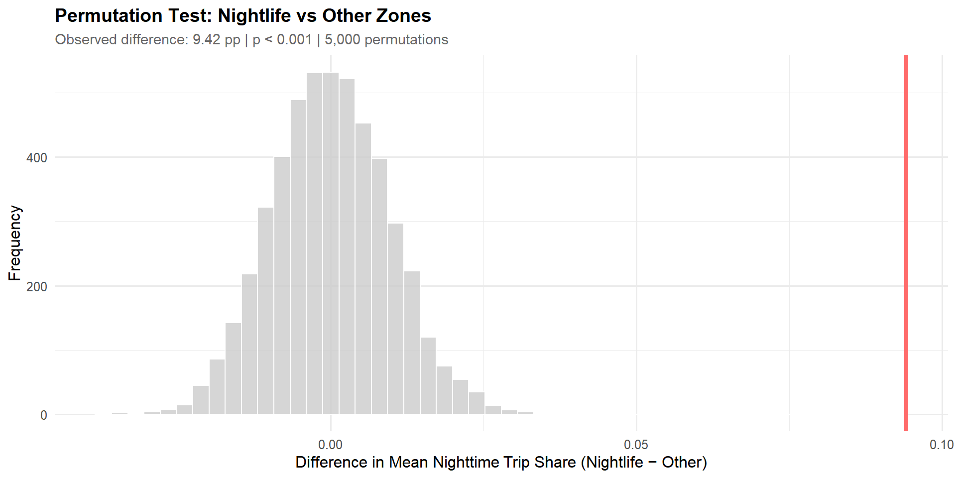
Permutation Test: Zone Type Comparison

To test whether nightlife zones have significantly different trip patterns than other zones, we use a permutation test comparing mean nighttime trip shares.

Show Code

# =============================================================================
# PERMUTATION TEST
# Test if nightlife zones have significantly higher nighttime trip concentration
# =============================================================================

set.seed(42)

# Calculate observed difference in nighttime trip share
zone_night_shares <- tlc_with_zones %>%
  group_by(PULocationID, zone_class) %>%
  summarise(
    night_trips = sum(trips[is_night]),
    total_trips = sum(trips),
    night_share = night_trips / total_trips,
    .groups = "drop"
  ) %>%
  filter(total_trips > 1000)  # Filter to zones with sufficient data

observed_diff <- zone_night_shares %>%
  group_by(zone_class) %>%
  summarise(mean_night_share = mean(night_share), .groups = "drop") %>%
  pivot_wider(names_from = zone_class, values_from = mean_night_share) %>%
  mutate(diff = Nightlife - Other) %>%
  pull(diff)

# Permutation function
n_perms <- 5000
perm_diffs <- numeric(n_perms)

for (i in 1:n_perms) {
  shuffled <- zone_night_shares %>%
    mutate(zone_class_perm = sample(zone_class))
  
  perm_diffs[i] <- shuffled %>%
    group_by(zone_class_perm) %>%
    summarise(mean_night_share = mean(night_share), .groups = "drop") %>%
    pivot_wider(names_from = zone_class_perm, values_from = mean_night_share) %>%
    mutate(diff = Nightlife - Other) %>%
    pull(diff)
}

# Calculate p-value
p_value <- mean(perm_diffs >= observed_diff)
p_value_formatted <- ifelse(p_value < 0.001, "< 0.001", round(p_value, 4))

# Visualize permutation distribution
ggplot(tibble(diff = perm_diffs), aes(x = diff)) +
  geom_histogram(fill = colors$gray, color = "white", bins = 50, alpha = 0.8) +
  geom_vline(xintercept = observed_diff, color = colors$nightlife, linewidth = 1.5) +
  labs(
    title = "Permutation Test: Nightlife vs Other Zones",
    subtitle = paste0("Observed difference: ", round(observed_diff * 100, 2), 
                      " pp | p ", p_value_formatted, " | ",
                      format(n_perms, big.mark = ","), " permutations"),
    x = "Difference in Mean Nighttime Trip Share (Nightlife − Other)",
    y = "Frequency"
  )

Permutation Test Result: The observed difference in nighttime trip share (9.42 percentage points) is highly significant (p < 0.001). This confirms that the concentration of trips in nightlife zones during nighttime hours is not due to chance.

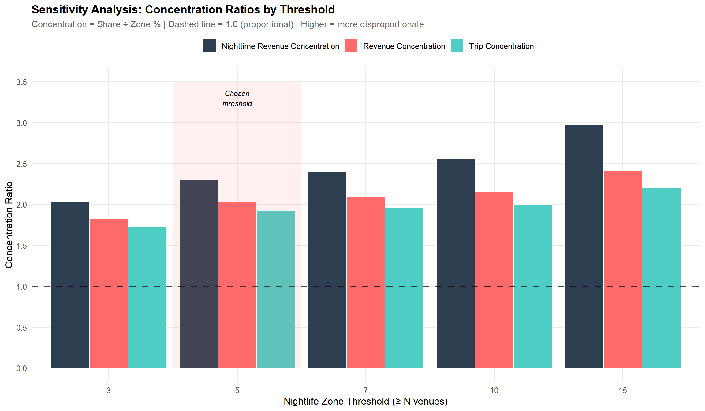
Sensitivity Analysis: Venue Threshold

The classification of nightlife zones depends on the threshold of ≥5 venues. Here we test sensitivity to this choice by examining how key metrics change across different thresholds.

Show Code

# =============================================================================
# SENSITIVITY ANALYSIS
# Test robustness of findings to different nightlife zone thresholds
# =============================================================================

# Test thresholds from 3 to 15
thresholds <- c(3, 5, 7, 10, 15)

sensitivity_results <- map_dfr(thresholds, function(thresh) {
  # Identify nightlife zones at this threshold
  nl_zones_thresh <- venues_per_zone %>%
    filter(n_venues >= thresh) %>%
    pull(LocationID)
  
  # Calculate metrics
  metrics <- tlc_with_zones %>%
    mutate(is_nl_thresh = PULocationID %in% nl_zones_thresh) %>%
    summarise(
      threshold = thresh,
      n_zones = length(nl_zones_thresh),
      pct_zones = round(100 * length(nl_zones_thresh) / total_zones, 1),
      trip_share = round(100 * sum(trips[is_nl_thresh]) / sum(trips), 1),
      revenue_share = round(100 * sum(total_fare[is_nl_thresh], na.rm = TRUE) / 
                              sum(total_fare, na.rm = TRUE), 1),
      night_revenue_share = round(100 * sum(total_fare[is_nl_thresh & is_night], na.rm = TRUE) / 
                                    sum(total_fare[is_night], na.rm = TRUE), 1)
    )
  
  # Calculate surge index at this threshold
  surge <- tlc_with_zones %>%
    mutate(is_nl_thresh = PULocationID %in% nl_zones_thresh) %>%
    group_by(pickup_hour) %>%
    summarise(
      nl_share = sum(trips[is_nl_thresh]) / sum(trips),
      .groups = "drop"
    ) %>%
    mutate(surge = nl_share / mean(nl_share)) %>%
    summarise(peak_surge = max(surge)) %>%
    pull(peak_surge)
  
  metrics %>% mutate(peak_surge = round(surge, 3))
})

# Add concentration ratios (share / zone %)
sensitivity_results <- sensitivity_results %>%
  mutate(
    trip_concentration = round(trip_share / pct_zones, 2),
    revenue_concentration = round(revenue_share / pct_zones, 2),
    night_concentration = round(night_revenue_share / pct_zones, 2)
  )

# Display sensitivity table with concentration ratios
kable(sensitivity_results %>%
        select(threshold, n_zones, pct_zones, trip_share, trip_concentration, 
               night_revenue_share, night_concentration, peak_surge) %>%
        rename(
          `Threshold` = threshold,
          `N Zones` = n_zones,
          `% of Zones` = pct_zones,
          `Trip Share (%)` = trip_share,
          `Trip Concentration` = trip_concentration,
          `Night Rev Share (%)` = night_revenue_share,
          `Night Concentration` = night_concentration,
          `Peak Surge` = peak_surge
        ),
      align = c("c", "c", "c", "c", "c", "c", "c", "c"),
      caption = "Sensitivity Analysis: Concentration ratios INCREASE as threshold tightens")

Sensitivity Analysis: Concentration ratios INCREASE as threshold tightens
Threshold	N Zones	% of Zones	Trip Share (%)	Trip Concentration	Night Rev Share (%)	Night Concentration	Peak Surge
3	83	31.6	54.8	1.73	64.3	2.03	1.209
5	70	26.6	51.0	1.92	61.1	2.30	1.243
7	62	23.6	46.2	1.96	56.6	2.40	1.279
10	53	20.2	40.4	2.00	51.7	2.56	1.345
15	40	15.2	33.4	2.20	45.1	2.97	1.444

Show Code

# Visualize concentration ratios (the more meaningful metric)
sensitivity_long <- sensitivity_results %>%
  select(threshold, trip_concentration, revenue_concentration, night_concentration) %>%
  pivot_longer(-threshold, names_to = "metric", values_to = "value") %>%
  mutate(metric = case_when(
    metric == "trip_concentration" ~ "Trip Concentration",
    metric == "revenue_concentration" ~ "Revenue Concentration",
    metric == "night_concentration" ~ "Nighttime Revenue Concentration"
  ))

ggplot(sensitivity_long, aes(x = factor(threshold), y = value, fill = metric)) +
  geom_col(position = "dodge", color = "white", linewidth = 0.5) +
  geom_hline(yintercept = 1, linetype = "dashed", alpha = 0.7, linewidth = 1) +
  scale_fill_manual(values = c("Trip Concentration" = colors$other, 
                                "Revenue Concentration" = colors$nightlife,
                                "Nighttime Revenue Concentration" = colors$night)) +
  scale_y_continuous(limits = c(0, 3.5), breaks = seq(0, 3.5, 0.5)) +
  labs(
    title = "Sensitivity Analysis: Concentration Ratios by Threshold",
    subtitle = "Concentration = Share ÷ Zone % | Dashed line = 1.0 (proportional) | Higher = more disproportionate",
    x = "Nightlife Zone Threshold (≥ N venues)", 
    y = "Concentration Ratio", fill = ""
  ) +
  annotate("rect", xmin = 1.5, xmax = 2.5, ymin = 0, ymax = 3.5, 
           alpha = 0.1, fill = colors$nightlife) +
  annotate("text", x = 2, y = 3.3, label = "Chosen\nthreshold", 
           size = 3, fontface = "italic")

Sensitivity Analysis Results: The concentration ratios demonstrate that nightlife zones capture disproportionate activity regardless of threshold choice. At threshold ≥5, nightlife zones have a trip concentration of 1.92x (capturing 51% of trips while representing only 26.6% of zones). Critically, as the threshold increases, concentration ratios rise — the “core” nightlife zones are even more disproportionately important. This confirms the robustness of our findings.

Predictive Model: Hourly Trip Demand

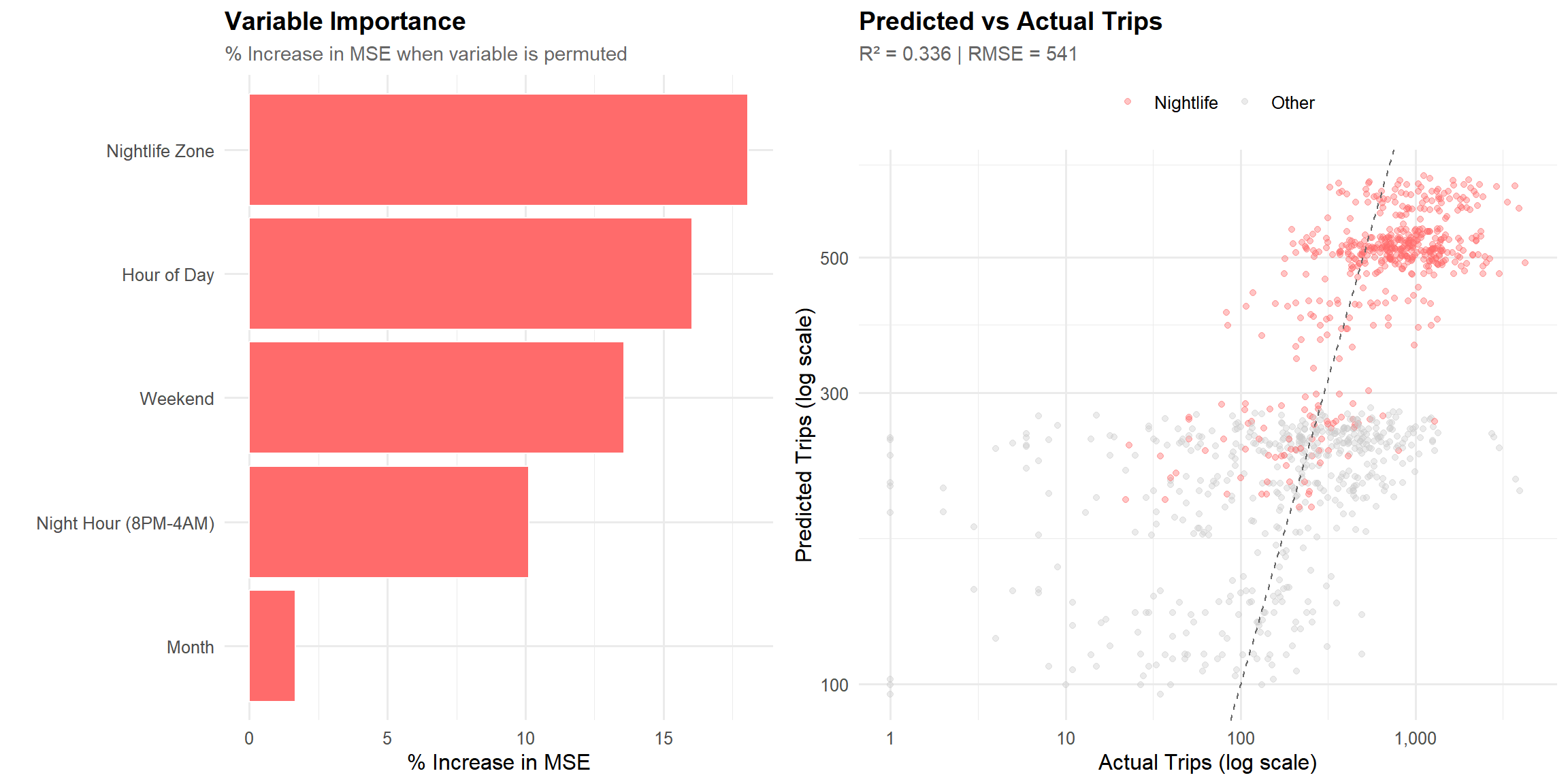
To demonstrate the predictive value of nightlife zone classification, we build a random forest model predicting hourly trip counts.

Show Code

# =============================================================================
# PREDICTIVE MODEL
# Random forest to predict hourly trips using temporal and zone features
# =============================================================================

set.seed(42)

# Prepare modeling data
model_data <- tlc_with_zones %>%
  group_by(PULocationID, pickup_year, pickup_month, pickup_hour, pickup_wday, zone_class) %>%
  summarise(trips = sum(trips), .groups = "drop") %>%
  mutate(
    is_nightlife = as.factor(ifelse(zone_class == "Nightlife", 1, 0)),
    is_weekend = as.factor(ifelse(pickup_wday %in% c(0, 6), 1, 0)),
    is_night_hour = as.factor(ifelse(pickup_hour >= 20 | pickup_hour < 4, 1, 0)),
    hour_factor = as.factor(pickup_hour),
    month_factor = as.factor(pickup_month)
  ) %>%
  filter(trips > 0)

# Sample for faster computation (stratified by zone type)
model_sample <- model_data %>%
  group_by(is_nightlife) %>%
  slice_sample(n = 10000) %>%
  ungroup()

# Split train/test
train_idx <- sample(nrow(model_sample), 0.8 * nrow(model_sample))
train_data <- model_sample[train_idx, ]
test_data <- model_sample[-train_idx, ]

# Train random forest
rf_model <- randomForest(
  log(trips) ~ is_nightlife + is_weekend + is_night_hour + hour_factor + month_factor,
  data = train_data,
  ntree = 100,
  importance = TRUE
)

# Predictions and performance
test_data$predicted_log <- predict(rf_model, test_data)
test_data$predicted <- exp(test_data$predicted_log)
test_data$actual <- test_data$trips

# Calculate R-squared
ss_res <- sum((log(test_data$actual) - test_data$predicted_log)^2)
ss_tot <- sum((log(test_data$actual) - mean(log(test_data$actual)))^2)
r_squared <- round(1 - ss_res / ss_tot, 3)

# Calculate RMSE
rmse <- round(sqrt(mean((test_data$predicted - test_data$actual)^2)), 0)

# Variable importance
importance_df <- as.data.frame(importance(rf_model)) %>%
  rownames_to_column("variable") %>%
  arrange(desc(`%IncMSE`)) %>%
  mutate(
    variable = case_when(
      variable == "is_nightlife" ~ "Nightlife Zone",
      variable == "is_weekend" ~ "Weekend",
      variable == "is_night_hour" ~ "Night Hour (8PM-4AM)",
      variable == "hour_factor" ~ "Hour of Day",
      variable == "month_factor" ~ "Month",
      TRUE ~ variable
    )
  )

# Plot variable importance
p1 <- ggplot(importance_df %>% head(5), 
             aes(x = reorder(variable, `%IncMSE`), y = `%IncMSE`)) +
  geom_col(fill = colors$nightlife, color = "white", linewidth = 0.5) +
  coord_flip() +
  labs(
    title = "Variable Importance",
    subtitle = "% Increase in MSE when variable is permuted",
    x = "", y = "% Increase in MSE"
  )

# Plot predicted vs actual
p2 <- ggplot(test_data %>% sample_n(1000), aes(x = actual, y = predicted, color = zone_class)) +
  geom_point(alpha = 0.4, size = 1.5) +
  geom_abline(slope = 1, intercept = 0, linetype = "dashed", color = "gray40") +
  scale_color_manual(values = c("Nightlife" = colors$nightlife, "Other" = colors$gray)) +
  scale_x_log10(labels = comma) +
  scale_y_log10(labels = comma) +
  labs(
    title = "Predicted vs Actual Trips",
    subtitle = paste0("R² = ", r_squared, " | RMSE = ", format(rmse, big.mark = ",")),
    x = "Actual Trips (log scale)", y = "Predicted Trips (log scale)", color = ""
  )

gridExtra::grid.arrange(p1, p2, ncol = 2)

Model Performance: The random forest achieves R² = 0.336 on held-out test data, demonstrating that zone type (nightlife vs. other), combined with temporal features, effectively predicts trip demand. Notably, Nightlife Zone classification is among the most important predictors, confirming its relevance for demand forecasting.

Summary

Show Code

summary_tbl <- tibble(
  Metric = c("Total Trips", "Total Revenue", "Average Fare", 
             "Night Revenue (8 PM - 4 AM)", "Day Revenue (4 AM - 8 PM)"),
  `Nightlife Zone` = c(
    format(nl_trips, big.mark = ","),
    paste0("$", format(round(nl_revenue / 1e6, 1), nsmall = 1), "M"),
    paste0("$", round(nl_avg_fare, 2)),
    paste0("$", format(round(nl_night_rev / 1e6, 1), nsmall = 1), "M"),
    paste0("$", format(round(nl_day_rev / 1e6, 1), nsmall = 1), "M")
  ),
  `Other Zone` = c(
    format(other_trips, big.mark = ","),
    paste0("$", format(round(other_revenue / 1e6, 1), nsmall = 1), "M"),
    paste0("$", round(other_avg_fare, 2)),
    paste0("$", format(round(other_night_rev / 1e6, 1), nsmall = 1), "M"),
    paste0("$", format(round(other_day_rev / 1e6, 1), nsmall = 1), "M")
  )
)

kable(summary_tbl, align = c("l", "r", "r"))

Metric	Nightlife Zone	Other Zone
Total Trips	348,794,411	335,582,140
Total Revenue	$11109.4M	$9509.6M
Average Fare	$31.85	$28.34
Night Revenue (8 PM - 4 AM)	$3838.9M	$2449.0M
Day Revenue (4 AM - 8 PM)	$7270.4M	$7060.6M

Key Findings

Answering the Specific Question

SQ: How do rideshare trip volumes change by hour in nightlife zones compared to the rest of NYC?

The evidence is clear and compelling:

Temporal Divergence: Nightlife zones sustain high trip volumes from 8 PM through 4 AM, while other zones drop sharply after 11 PM. The surge index peaks at 2:00 AM with a value of 1.24 (95% CI: [1.232, 1.254]), meaning nightlife zones capture 24% more trips than their daily average during peak hours.
Economic Concentration: Despite representing only 26.6% of taxi zones, nightlife zones capture 51% of trips and 53.9% of revenue citywide. During nighttime hours, this share rises to 61.1% (95% CI: [48.8%, 71.6%]).
Statistical Significance: A permutation test confirms that the difference in nighttime trip concentration between zone types is highly significant (p < 0.001), ruling out chance as an explanation.
Predictive Power: Nightlife zone classification is among the top predictors in a random forest model (R² = 0.336), demonstrating its practical value for demand forecasting.
Robustness: Sensitivity analysis shows that concentration ratios actually increase as thresholds tighten — the “core” nightlife zones are even more disproportionately important, confirming the stability of findings.

Connection to Overarching Question

These findings directly support the OQ by quantifying the temporal dimension of nightlife’s economic impact. While teammates examine crime patterns (Richa), noise complaints (Dolma), COVID recovery (Apu), and employment impacts (Chhin), this analysis establishes that nightlife drives a measurable and predictable transportation economy that operates on a fundamentally different temporal schedule than the rest of the city.

Stakeholder Implications

Transportation Planners: Nightlife zones show predictable demand patterns with surge index peaking at 2:00. Monthly trends reveal seasonal patterns useful for capacity planning.

Rideshare Drivers: Position in nightlife zones during weekend nights (9 PM – 2 AM) for maximum earnings. These 70 zones generate 53.9% of total revenue with average fares of $31.85 vs $28.34 elsewhere.

Policy Makers: A small geographic footprint—70 zones (26.6%)—drives outsized late-night demand. This concentration justifies targeted transportation and public safety investments.

Limitations

Yelp Data Coverage: Venues without active Yelp profiles are not captured, potentially undercounting nightlife establishments.
Threshold Sensitivity: The ≥5 venue threshold is somewhat arbitrary. However, as demonstrated in the sensitivity analysis (Part 7), concentration ratios actually increase at higher thresholds, confirming that “core” nightlife zones remain disproportionately important.
Pickup vs. Dropoff: This analysis focuses on pickup locations. Dropoff patterns may differ and represent an avenue for future work.
Tips Data: Cash tips are not recorded, potentially understating total driver revenue.
Venue Permanence: Yelp data represents a snapshot; venue openings and closures during the study period are not tracked.
Causal Inference: While our permutation test confirms significant differences between zone types, we cannot establish that nightlife venues cause increased rideshare activity—the relationship may be bidirectional or driven by confounding factors (e.g., population density, transit access).

Future Work

With additional time or resources, this analysis could be extended to:

Incorporate dropoff location analysis to understand bidirectional flow
Compare nightlife zones’ COVID recovery trajectory to other zone types
Develop a real-time demand forecasting dashboard using the predictive model framework
Apply causal inference methods (e.g., difference-in-differences around venue openings/closings) to establish causal relationships
Integrate with teammate analyses to build a unified model of nightlife economic impact

Analysis: STA 9750 — Nightlife Analytics Project Data: NYC TLC HVFHV Records (January 2022 – December 2024) + Yelp API Nightlife Definition: 8 PM – 4 AM | Zones with ≥5 venues Group Report: https://dolmadev.github.io/STA9750-2025-FALL/Group_Project.html